Multiple object tracking

2024-04-07
Per Halvorsen
GitHub
LinkedIn

In this note is meant to serve as a compendium of resources for multiple object tracking. It can be interpreted as a work-in-progress, with the intention to be expanded upon as more resources arise.

Previous notes on this topic are Exploring the Monterey Bay Benthic Object Detector and Applying Super-resolution to MBARI Benthic Object Detector.

Overview

• Background

  • Object detection
  • Object tracking

• Tools for tracking

  • Classic CV techniques
    • Segmentation
      • Background subtraction
      • Contour detection
      • Mean-shift filtering
    • Association
      • Hungarian algorithm
      • Kalman filter
      • Mahalanobis distance
  • Modern techniques
    • SORT
    • DeepSORT
    • ByteTrack

• Implementation

  • ByteTrack (Roboflow)

Background

Object detection

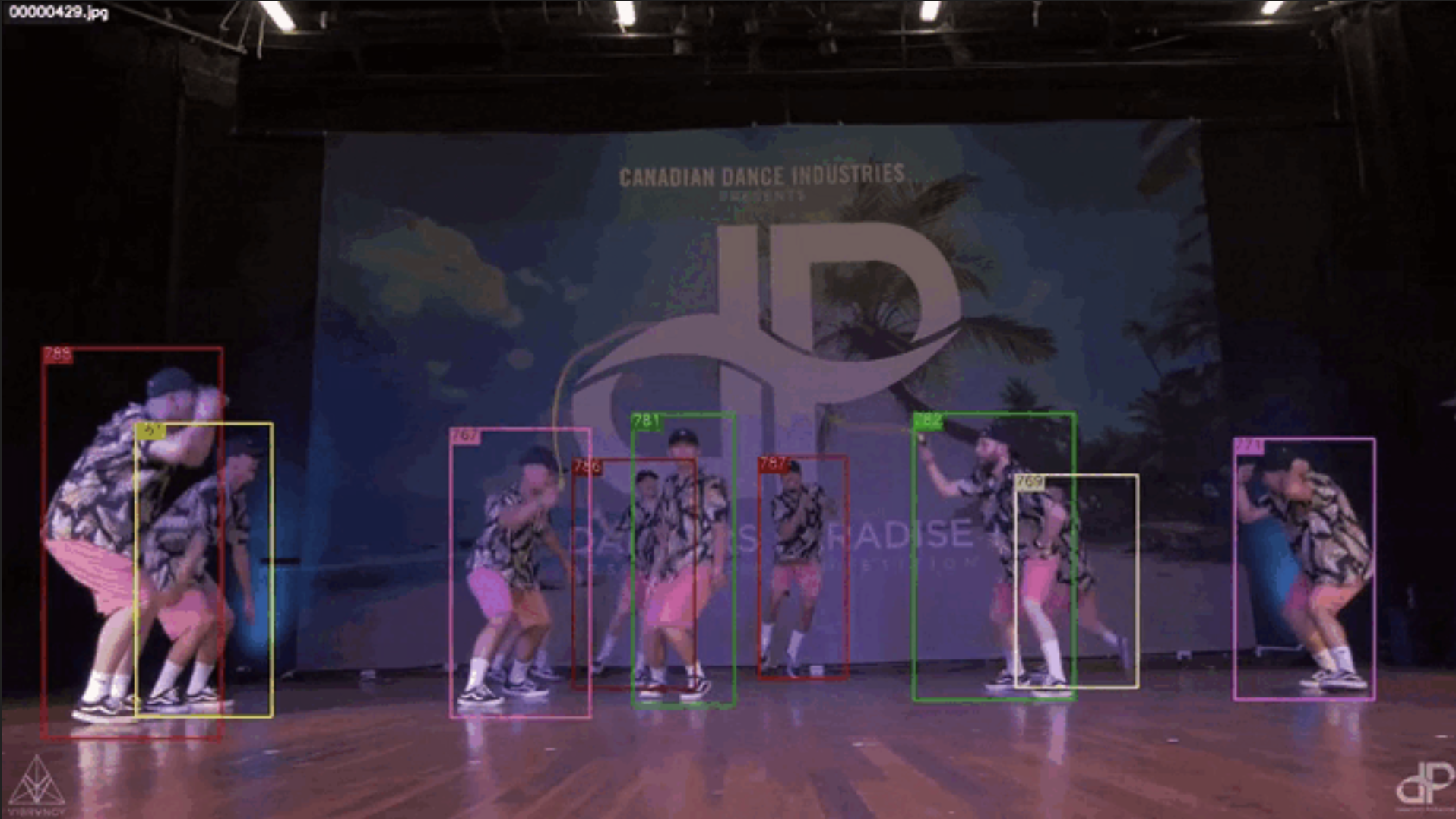
Figure 1: Example of object detection of a frame from a dance video (Dataset, Detector)

In object detection, a single frame is considered in isolation, and the goal is to identify and classify particular objects in the frame by drawing bounding boxes around them. This can be done with a focus on a single object or multiple objects, depending on model objective, complexity, and available compute resources. Detections are usually thresholded by a confidence score, and non-maximum suppression is applied to remove overlapping boxes. To achieve state-of-the-art performance on object detection alone, new architectures will likely be focused more on prediciton correctness rather than speed.

Some of the most polular object detection models include YOLO (maintained by Ultralytics) and Faster R-CNN. A state-of-the-art leader board for object detection models can be found on the Papers with Code website here. There, you can find the most recent models, along with their whitepapers and code implementations.

Object tracking

Figure 1: Example of object tracking in a dance video. (Source: github.com/noahcao/OC_SORT)

Object tracking builds off object detection, but it considers multiple frames in a video sequence. The goal is to associate detections across frames to track the same object over time. In these cases, speed is often more important than initial correctness, as the model must process many frames in a video sequence. The model must consider the object's movement, occlusion, and appearance changes, and update it's detection and tracking accordingly.

Typically, it is useful for these models to assign a unique ID to each object in the video sequence. A good tracker will be able to maintain the same ID for an object even when it is occluded or changes appearance. For more rudimentary tracking methods, re-identifying tracked objects occluded by other objects can be a challenge. This may result in the same object receiving new IDs after reappearance, or the object being lost entirely.

Modern trackers exploit deep learning components to include more temporal or visual information about the detections to assist in this process. These more complex trackers can be slower or require more compute resources, introducing a trade-off between speed and correctness. Decisions around this trade-off will depend on the specific use case and available resources.

Tools for tracking

With a brief overview of object tracking as a task, we can now explore some techniques in more detail.

Classic

Tradional computer vision techniques can be applied to videos as light-weight trackers. Below are a list of some of the most popular classic tracking algorithms, along with breif explanations and links to blog posts explaining further. These simplified set-ups will require two main steps: object segementation and object association.

Segmentation

Background detection

While not directly a tracking algorithm, background detection can be used in tandem with other traditional computer vision techniques to make up a light-weight tracker. The general idea is to determine a static background from a set of frames, to differentiate these pixels from moving objects.

A video's background can be determied as the median pixel values for all frames, a process known as temporal median filtering. Such a technique assumes few moving objects and a static background, where moving objects are present in any given pixel in less than 50% of the frames. This method is rudimentary but can be effective in simple tracking tasks, video surveillance, and other applications where the background is relatively static.

More details on background estimation can be found in this blogpost on Simple Background Estimation in Videos using OpenCV.

Contour detection

Before the wide-spread use of neural networks, one way of detecting edges in an image was to use greyscales and binary thresholding. An input image could be converted to greyscale, removing any superfluous color information. Then, a binary threshold is applied to the greyed image, where pixel values above a certain threshold are set to 1, and those below are set to 0. The result was then a binary image, where edges were represented by the transition from 0 to 1. Here, a simple contour detection algorithm can be applied to trace the pixels along the edges of objects in the image.

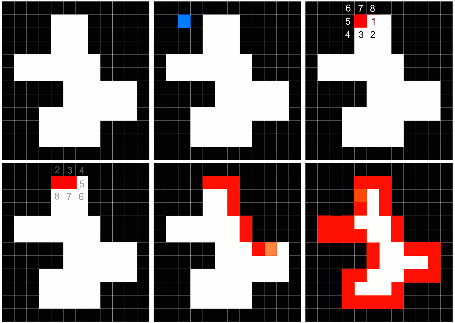
Example of contour detection in OpenCV. (Source: learnopencv.com)

This simple yet useful approach can be applied to videos with both static and dynamic background. The setup requires minimal computational resources and can therefore can be implemented in various stages of a pipelines. In preprocessing steps, contour detection can assist in object detection, telling a model where in a frame it should focus most, increasing detection and segmentation performance. Additionally, contour detection can help in post-detection stages to assist in association and tracking, when combined with IOU or other metrics.

A very simple tracker could be build by using contour detection to segment objects in a frame, labeling each segmented object with an id. The "detection" step can be quickly run for each frame, recalculating the detections and labels for each frame. However, in videos where new objects appear or objects disappear, these labels will differ, thus requiring more complex logical around label association between frames. This topic will be explored more thoroughly in the section titled Association.

A detailed walk-through implementing contour detection can be found here.

Mean-shift clustering/segmentation

Similar to K-means clustering, mean-shift clustering is a method for finding the modes (or segmentations) of a distribution of data points.

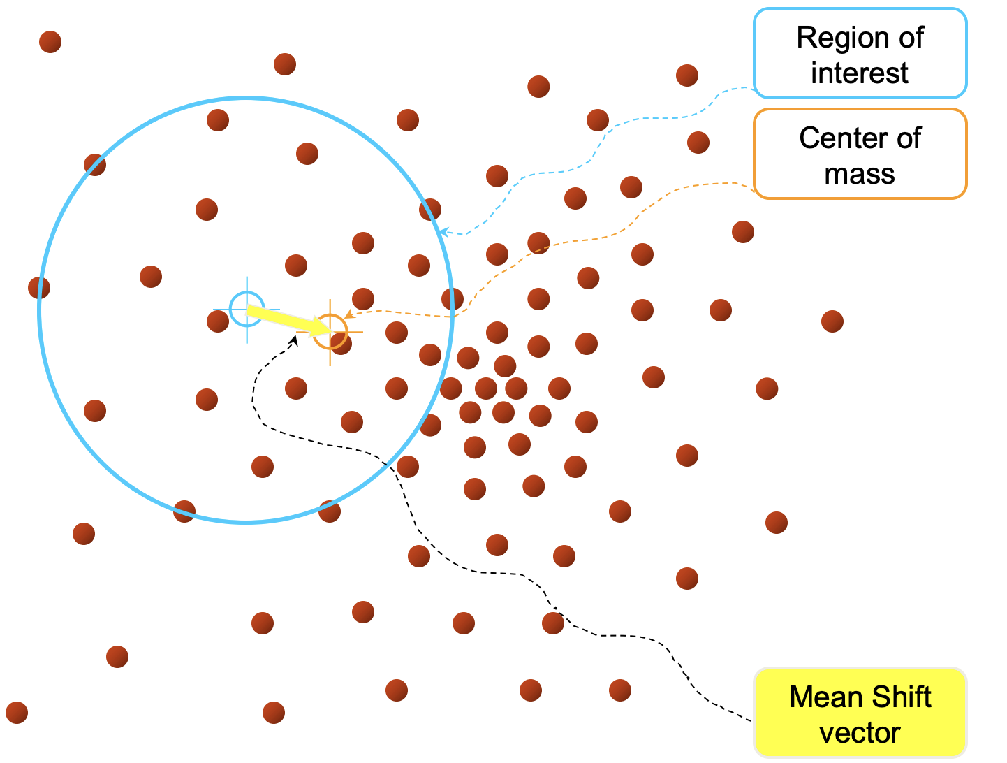
Example of mean-shift clustering in a 2D feature space. (Source: Stanford Vision and Learning Lab)

The algorithm starts by tessellating the feature space with a grid of windows, each centered on a pixel (i.e. odd numbered height and width window sizes). The algorithm then shifts each window to the mean of the data points, based on the selected feature space. Eventually, the windows will converge around a single point, which is considered a mode or peak in the data distribution. Windows that converge near the same peak are then merged, and the process is repeated until all windows have converged.

In a simplfied 1D set-up (i.e. a greyscale image), the feature space could be the pixel intesity, between 0 and 255. For colored image segmentation, one could instead use the RGB values of an input image. For an even more complex set-up, the feature space could be a combination of pixel color, texture, or other means of describing a subregion of an image.

Similar to contour detection, mean-shift clustering can be used in both pre- and post-processing stages of a pipeline, helping extract the mos timportant features of an input image. A great resource for understanding both mean-shift filtering and k-means filtering (skipped in our note) can be found in this lecture from Stanford Vision and Learning Lab.

Association

Kalman filter (SORT)

While not exactly an association technique by itself, Kalman filters are often used together with association funcitons like the Hungarian algorithm to update estimations about an object's position. The Kalman filter is a recursive algorithm that estimates the state of a linear dynamic system from a series of noisy measurements. It is used in many fields, including robotics, computer vision, and economics, to predict the future state of a system based on its past states.

The Kalman filter is based on two main assumptions:

1. The state of the system can be represented as a linear dynamic system.
2. The noise in the system is Gaussian, representable via a mean about 0 and an unknown variance.

By a linear dynamic system, we mean that the state of the system at the next time step can be predicted based on the previous state and the system's dynamics (velocity and direction). The step-functions are considered constant, and the system's estimated state can be predicted based on these constants, similar to a derivative-based physics simulation using $\frac{\delta x}{\delta t}$.

The Kalman filtering can be broken down into 3 main stages:

1. Estimatation: Estimate the current state of the system based on the fixed velocity and (randomly initialized) direction $\rightarrow \hat x_{t+1}$
2. Detection: Make a (noisy) measurement of the system $\rightarrow y_{t+1}$
3. Update: Update the state estimate with information of the new measurement, giving a more accurate prediction of the system's state $\rightarrow x_{t+1}$

One of the reasons Kalman filters are so useful is because they make use of all the information available to the system. The more information available to a system, the less uncertainty, and thus the more accurate the predictions.

Kalman filters are often used in tracking applications to predict the object's position based on its velocity and update the position based on the detection. The Simple Online Realtime Tracking (SORT) algorithm is a popular tracking algorithm that uses Kalman filtering for predictions and the Hungarian algorithm for association.

A really great resource for understanding Kalman filters is this YouTube video by Visually Explained. A hand-written note covering some of these topics can also be found in this repository here.

Hungarian algorithm (SORT)

The Hungarian algorithm is a combinatorial optimization algorithm that solves the assignment problem in polynomial time. It uses a cost matrix to find the optimal assignment of objects across frames, minimizing the total cost of the assignment. The metric used to calculate the cost can be the intersection over union (IOU) between the detections in two frames, the Euclidean distance between the detections, or another metric that captures the similarity between the detections.

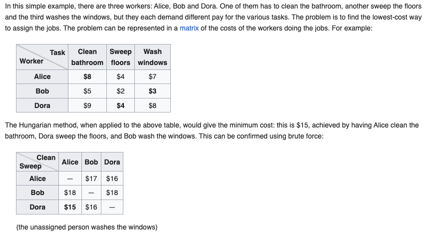
Example of the Hungarian algorithm in action on a small example. (Source: Wikipedia)

The steps needed to achieve this systematically are as follows:

1. Subtract the smallest element in each row from all elements in that row
2. Subtract the smallest element in each column from all elements in that column
3. Draw the minimum number of lines needed to cover all zeros in the matrix
4. If the number of lines drawn equals the number of rows, the optimal assignment is found
5. If not, find the smallest element not covered by a line and subtract it from all uncovered elements, and add it to all elements covered by two lines
6. Repeat steps 3-5 until the optimal assignment is found

The Hungarian algorithm is used in the SORT algorithm to find the optimal assignment of detections across frames, minimizing the total cost of the assignment. Since the Hungarian algorithm is inherently designed to minimize a cost matrix, the input cost matrix to the algorithm is designed to minimize the negative of the IOU between detections in two frames. This way, the Hungarian algorithm will find the optimal assignment of detections that maximizes the IOU between the detections.

Think Autonomous has great blog-post for applying the Hungrian algorithm to object tracking. There you can find an even more detailed break down of each of the steps mentioned above, along with clear video and examples of different cost metrics used in the algorithm.

Mahalanobis Distance

The Mahalanobis distance is a measure of the distance between a point and a distribution of other data points, introduced by P. C. Mahalanobis in 1936. It is a multi-dimensional generalization of the idea of measuring how many standard deviations away the point is from the mean of the distribution. This distance is zero if the observed point is at the mean of distribution (think the center of a circle or centroid of an ellipse), and grows as the point moves away from the mean along each principal component axis.

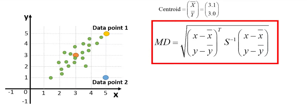
Example of the Mahalanobis distance in a 2D feature space. (Source: TileStats (YouTube))

The example above comes from a video comparing the Euclidean distance to the Mahalanobis distance in a 2D feature space. In the image we see, the Euclidean distance between the distribution mean and the two data points is the same, while the Mahalanobis distance is different. The Mahalanobis distance takes into account the covariance of the data, which provides information on the trend of the distribution (diagonally in this case).

In a sense, the Mahalonobis distance mixes the concepts of the mean-shift algorithm mentioned above with information about the covariance of the data. Taking into account the covariance of the data allows the metric to account for the correlations between the data, which can be useful in tracking applications where the location of an object can change in both the x and y directions. An object moving along a path will more likely continue along that path, rather than suddenly change direction. The Mahalanobis distance can account for this expected path continuation, and thus provide a more accurate measurement of the distance between a detected object and its previous occurances.

In modern object trackers, the Mahalanobis distance sometimes replaces the IOU metrics in associations steps between the predicted bounding boxes and the ground truth bounding boxes, as in Deep SORT. For more information on the Mahalanobis distance, check out the video by TileStats mentioned above.

Modern

SORT

We've already mentioned the Simple Online Realtime Tracking (SORT) (A. Bewley et. al. 2016) algorithm a few times now, but can coalesce the information here. This algorithm is a simple, yet effective, tracking algorithm that uses a Kalman filter for state estimation and the Hungarian algorithm for association. SORT is an online tracking algorithm, meaning it processes frames one at a time and does not require the entire video to be loaded into memory.

For each frame, SORT performs the following steps:

1. Detection: Run an object detector on the current frame to get the detections
2. Esimation: Make a best estimate of the state of the object in the next frame using a Kalman filter
3. Association: Use the Hungarian algorithm to associate the detections across frames
4. Create & Delete: Create new tracks for unmatched detections and delete old tracks that have not been matched for a certain number of frames

The methodology section of the original SORT paper actually does a great job at explaining the algorithm in detail, so I would recommend reading that if you want to learn more about SORT. Implementations of SORT can be found in the original repository github.com/abewley/sort. You can also refer to my handwritten note diving into more of the math around SORT and Kalman filtering.

DeepSORT

DeepSORT (N. Wojke et. al. 2017) is an extension of the SORT algorithm that uses deep learning to improve tracking performance. The main difference between SORT and DeepSORT is that DeepSORT uses a deep neural network to extract embeddings from the detections, which are then used to associate the detections across frames. This allows DeepSORT to associate objects across frames even when they are occluded or change appearance.

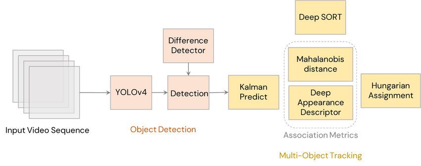
Overview of DeepSORT. (Source: A. Parico et. al. (2021))

The embeddings are learned representations of the object's appearance that are used to associate objects across frames. They are learned by training a deep neural network on a large dataset of images with labeled objects. For optimal performance, the embeddings should likely be fine-tuned to the domain on which the tracker will be used.

The DeepSORT algorithm can be broken down into the following steps:

1. Detection: Run an object detector on the current frame to get the detections getting the bounding boxes and confidence scores for each detection.
2. Feature extraction: For each detected object, use a deep neural network to extract embeddings representing the object's appearance.
3. Estimation: Make a best estimate of the state of the object in the next frame using a Kalman filter (similar to in SORT).
4. Association: Use the Hungarian algorithm to associate the detections across frames based on the embeddings. Instead of an IOU metric, the vallues of the cost matrix are the Mahalanobis distances between object locations and a cosine similarity of the appearance embeddings.
5. Create & Delete: Create new tracks for unmatched detections and delete old tracks that have not been matched for a certain number of frames
6. Re-identification: Re-identify objects that have been occluded or changed appearance by comparing the embeddings of the detections.

The (italicized) novel steps the DeepSORT algorithm introduces are the feature extraction step, the Mahalanobis distance in association step, and re-identification step. The feature extraction and re-id steps are the introduction of deep learning components to the SORT algorithm, which allows DeepSORT to associate objects across frames even when they are occluded or change appearance.

Implementations of DeepSORT can be found in the original repository github.com/nwojke/deep_sort.

ByteTrack

ByteTrack (Y. Zhang et. al. 2021) is a recent object tracking algorithm that builds off many of the conecpts of SORT and DeepSORT, but introduces the concept of using both high and low-confidence detections to improve tracking performance. The algorithm is designed to be lightweight for fast and efficient tracking, making it suitable for real-time applications.

The steps of the ByteTrack model can be outlined as follows:

1. Detection: Utilizes an object detector like YOLO to predict detection boxes and scores for each frame in a video sequence.
2. Confidence Categorization: Separates the detection boxes into high-confidence and low-confidence subsets based on a predefined score threshold.
3. Estimation: Applies the Kalman filter to estimate the new locations of tracks in the current frame, capturing the object's motion similar to SORT and DeepSORT.
4. High-Confidence Association: Associates high-confidence detection boxes with existing tracks using algorithms like the Hungarian algorithm for initial matching. Here, either the slightly modified IOU metric or the re-identification feature distances (cosine similarities) are used to calculate the cost matrix.
5. Low-Confidence Association: Incorporates low-confidence detections with existing tracks, improving the ability to maintain track continuity even with partially occluded objects. Here, only the IOU metric is used to calculate the cost matrix, as the re-id features may be obscured, hence producing a lower confidence around the detection.
6. Create & Delete: Similar as before, create new tracks for unmatched high-confidence detections and delete tracks that are no longer visible or have insufficient evidence in the frames.

ByteTrack introduces the differing uses of the high and low-confidence detections, which significantly reduces missed detections and fragmented trajectories often caused by occlusions or poor visibility. Combining the concept of confidence handling together with the Kalman filter, the tracker has been able to improve benchmarked tracking performance without sacrificing speed or efficiency.

Implementations of ByteTrack can be found in the original repository github.com/ifzhang/ByteTrack and the white paper on arXiv. Roboflow has a great tutorial on how to implement ByteTrack with YOLOv5, which we will use in the next setion on implementation.

Implementation

ByteTrack (Roboflow)

In this section, we will walk through how to implement the ByteTrack algorithm using the YOLOv5 object detector. here, we can leverage the aforementioned tutorial from Roboflow to guide us through the process. This tutorial makes use of the supervision library to easily load in the ByteTracker tracking algorithm.

Since we do not currently have a lot of local computational resources, we will keep this implementation rather simple. With a working worklfow in place, we can later expand on the concepts presented here by distributing the model through Dockerized containers.

Imports

We will pip install the required libraries for our simple implementation of ByteTrack. Since we still want to use the Benthic Object Detector from MBARI, we will also need to ensure that the model weights are downloaded locally.

# # if you don't have them already, download supervision and torch  
# !pip install supervision torch -q 
# !pip install -q moviepy

from moviepy.editor import VideoFileClip
from IPython.display import Image

import numpy as np
import os
import supervision as sv
import torch


MODEL_PATH = "../../models/fathomnet_benthic/mbari-mb-benthic-33k.pt"
# model = torch.hub.load('ultralytics/yolov5', 'custom', path=model_name,  force_reload=True)

In order to testour tracker properly, we need to gather in some video data, where we know the true classifications. Using the screen_capture.py script found in src/tools/, we scraped some short clips of animals from different sources on YouTube. We can use these clips to manually evaluate the performance of the YOLOv5 + ByteTrack pipeline. They get stored locally in the data/ directory.

Some of the sources for videos we scraped include:

• Monterey Bay Aquarium
• Deep Marine Scenes
• EVNatilus

ByteTrack (default)

We can start by running the default ByteTrack model on a video clip of a sea feather, otherwise known as a Crinoidea. The sample clip can be found at data/example/sea_feather.mp4.

class YOLOv5_ByteTracker:

    def __init__(self, model_path=MODEL_PATH, **tracker_params):
        self.model = torch.hub.load('ultralytics/yolov5', 'custom', path=model_path,  force_reload=True)
        
        self.init_tracker(**tracker_params)  # create self.tracker and self.suffix attributes

        self.box_annotator = sv.BoundingBoxAnnotator()
        self.label_annotator = sv.LabelAnnotator()


    def init_tracker(self, **tracker_params):
        """Update the tracker parameters."""
        # for systematic naming of output files
        self.suffix = "_".join([f"{k}{v}" for k, v in tracker_params.items()]) if tracker_params else None

        self.tracker = sv.ByteTrack(**tracker_params)


    def callback(self, frame: np.ndarray, index: int) -> np.ndarray:
        """Detection callback callled for each frame in the video. Used in process_video later"""

        # frame = super_resolution_model(frame)  # TODO add when ready
        results = self.model(frame) #[0]
        detections = sv.Detections.from_yolov5(results)
        detections = self.tracker.update_with_detections(detections)
        labels = [
            f"#{tracker_id} {self.model.model.names[class_id]} {confidence:0.2f}"
            for bbox, _, confidence, class_id, tracker_id, _
            in detections
        ]
        frame = self.box_annotator.annotate(scene=frame.copy(), detections=detections)
        frame = self.label_annotator.annotate(scene=frame.copy(), detections=detections, labels=labels)
        return frame


    def mot(self, name, data_dir="../data/example", output_dir="../data/results", ext="mp4"):
        """Apply the MOT callback to a video and save the result to a new file."""
        output_name = name.split("/")[-1] if "/" in name else name
        if self.suffix:
            output_name += f"_{self.suffix}"
        
        sv.process_video(
            source_path=f"{data_dir}/{name}.{ext}", 
            target_path=f"{output_dir}/{output_name}_mot.{ext}", 
            callback=self.callback
        )

        return f"{output_dir}/{output_name}_mot.{ext}"


    def vid2gif(self, video_path, gif_path):
        """Convert a video to a gif."""
        clip = VideoFileClip(video_path)
        clip.write_gif(gif_path)
        return gif_path


    def mot_show(self, name, data_dir="../data/example", output_dir="../data/results", ext="mp4"):
        """Wrapper to display the result of the MOT callback as a gif."""
        mot_output_path = self.mot(name, data_dir, output_dir, ext)
        gif_output_path = self.vid2gif(mot_output_path, mot_output_path.replace(".mp4", ".gif"))

        # display the gif
        return Image(filename=gif_output_path)


tracker = YOLOv5_ByteTracker(MODEL_PATH)
tracker.mot_show("sea_feather") 

Downloading: "https://github.com/ultralytics/yolov5/zipball/master" to /Users/per.morten.halvorsen@schibsted.com/.cache/torch/hub/master.zip
YOLOv5 🚀 2024-4-7 Python-3.11.8 torch-2.2.2 CPU

Fusing layers... 
Model summary: 476 layers, 91841704 parameters, 0 gradients
Adding AutoShape... 

MoviePy - Building file ../data/results/sea_feather_mot.gif with imageio.

<IPython.core.display.Image object>

Crinoidea example footage from the Deep Marine Scenes YouTube channel.

As can be seen in the gif above, our out-of-the-box tracker worked quite well on our example video.

ByteTrack parameters

The supervision.ByteTrack class comes with a few tunable parameters. These include:

• track_activation_threshold: the confidence threshold for detections
• lost_track_buffer: a buffer or number of frames to keep tracking id alive when no detections for that object
• minimum_matching_threshold: the minimum similarity score (IOU or cosine-sim) for matching detections across frames
• frame_rate: the frame rate of the video

By adjusting these, we can see how the model detections can lead to very different tracking results.

Let's see want happens when we start tuning the parameters. To start, let's increase the confidence threshold needed to activate a track (default value here is 0.25).

tracker.init_tracker(track_activation_threshold=0.4)
tracker.mot_show("sea_feather") 

MoviePy - Building file ../data/results/sea_feather_track_activation_threshold0.4_mot.gif with imageio.

<IPython.core.display.Image object>

Notice how the tracker now has a harder time keeping track of the sea feather. At some point, detections are no longer confident enough to be consider worth tracking. Let's find a middle ground between the two thresholds.

tracker.init_tracker(track_activation_threshold=0.29)
tracker.mot_show("sea_feather") 

MoviePy - Building file ../data/results/sea_feather_track_activation_threshold0.29_mot.gif with imageio.

<IPython.core.display.Image object>

Notice how there are a few frames now where the tracker loses the sea feather and removes teh bounding box, but then quickly recovers it after about 2-3 frames. Its especially interesting here to look at the ID shown in the top left corner of the bounding box. This the is the unique tracked object ID stored internally in thre tracker.

If an object with similar appearance is detected later, and that ID's lost buffer hasn't expired, the tracker will assign the object the same id as before, as seen above. This re-identification is possible thanks to the deep learning embeddings used in the ByteTrack algorithm.

If the lost buffer expires however, the tracker will assign a new ID to the object, as seen in the gif above. Let's now adjust the lost buffer from its default value at 30 frames to a single frame, to see this new ID assignment in action. We will need to use the same confidence threshold as before, since that was the one that lost the object for a few detections in a row.

tracker.init_tracker(track_activation_threshold=0.29, lost_track_buffer=1)
tracker.mot_show("sea_feather") 

MoviePy - Building file ../data/results/sea_feather_track_activation_threshold0.29_lost_track_buffer1_mot.gif with imageio.

<IPython.core.display.Image object>

We now see that the tracker lost the sea feather, which later gets classified as an anemone, specifically a Bolocera. This highlights the importance of the leway given by the lost buffer, as it allows the tracker to re-identify objects that were occluded or changed appearance.

Another potential problem that can arise here is prolonged misclassifications of objects. If the inital detection is incorrect, the tracker may continue to track the object as if it were the misclassified object, even when the object detector has corrected itself.

This potential flaw in our pipeline might be fixed by tuning the minimum matching threshold, which is a threshold (IOU or cosine-similarity score) for matching detections across frames. In the documentation, it states that high values here will increase accuracy, but may lead to more fragmented tracks, while lowering would improve compleness but may lead to more false positives. Initial experimentation seems the opposite from what is documented (lower values give high fragmentation while higher values give little to no change). We will reserve looking further into this metric for future work, where we can test on a wider variety of videos and objects. Though we will not test this parameter here, it is important to keep in mind when tuning the tracker for your specific use case.

Conclusion

As can be inferred from the small experimentation ran above, the parameters of the tracker can be quite fragile

If the confidence threshold is too high, the tracker may lose objects that are still visible in the video. However, if the confidence is too low, the tracker may assign wrongly identify an object and stick with that misclassification for the rest of the video.

If the lost buffer is too low, the tracker may assign new IDs to objects that are still visible in the video. Though, if the buffer is too high, the tracker make have re-identifying objects that were difficult to predict for a few frames due to pose changes and occlusions.

Feel free to experiment with these parameters on your own, and see how they affect the tracking performance of the ByteTrack algorithm.

Extra resources

If you want to use screen_capture.py to scrape clips from the web on your end, you can easily run tracking on resulting videos using the below code:

# i = 0  # change this to the video you want to process
# tracker.mot_show(f"aquarium_{i:03}/aquarium_{i:03}", data_dir="../data/video", output_dir="../data/results", ext="mp4") 

Disclaimer

We must admit, it took a few tries before getting footage that actually had decent tracking results. The quality of the footage, the frame rate, the number of objects in the frame, and the object's movement all play a role in the tracking performance. This means the example chosen above was a bit cherry-picked to show the best results.

In a real-world scenario, the tracker may not perform as well as shown here, and may require more tuning to get the desired results. However, the main focus here was to get a reasonable tracking for an object obviously classifiable to the human eye.

Up next: Dockerizing our pipeline

With a working implementation in place, we can move on to the next step in this project, namely model distribution and deployment. Follow along on that development in PR#3.